6 Easy Facts About Excel Jobs Explained

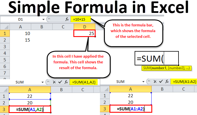
By pressing ctrl+change+center, this will certainly compute and return value from multiple varieties, instead of just private cells added to or increased by each other. Computing the sum, product, or quotient of private cells is very easy-- just utilize the =SUM formula and enter the cells, values, or variety of cells you desire to do that math on.

If you're looking to find overall sales revenue from a number of sold systems, as an example, the array formula in Excel is excellent for you. Below's how you 'd do it: To start utilizing the selection formula, kind "=SUM," and also in parentheses, go into the very first of 2 (or 3, or 4) varieties of cells you would certainly like to multiply with each other.

This means reproduction. Following this asterisk, enter your second series of cells. You'll be multiplying this 2nd series of cells by the initial. Your development in this formula should now look like this: =AMOUNT(C 2: C 5 * D 2:D 5) Ready to press Go into? Not so fast ... Since this formula is so challenging, Excel reserves a various keyboard command for varieties.

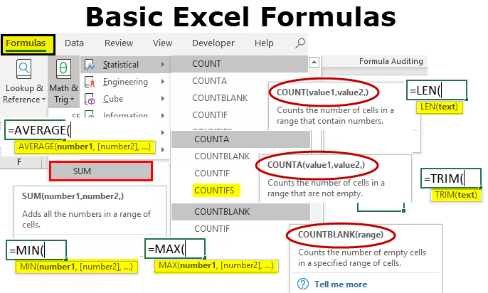
This will certainly identify your formula as an array, wrapping your formula in brace personalities and also efficiently returning your item of both arrays integrated. In income computations, this can cut down on your effort and time dramatically. See the final formula in the screenshot above. The MATTER formula in Excel is denoted =COUNT(Start Cell: End Cell).

For instance, if there are 8 cells with gone into values in between A 1 as well as A 10, =COUNT(A 1: A 10) will return a value of 8. The COUNT formula in Excel is especially helpful for large spread sheets, in which you intend to see the number of cells contain actual entrances. Do not be tricked: This formula won't do any type of mathematics on the worths of the cells themselves.

The Ultimate Guide To Countif Excel

Utilizing the formula in bold above, you can conveniently run a count of current cells in your spreadsheet. The result will certainly look a something like this: To carry out the average formula in Excel, enter the values, cells, or series of cells of which you're calculating the average in the layout, =STANDARD(number 1, number 2, etc.) or =STANDARD(Begin Value: End Value).

Finding the standard of an array of cells in Excel keeps you from needing to discover private sums and afterwards doing a different department formula on your overall. Using =STANDARD as your first text entry, you can allow Excel do all the help you. For recommendation, the average of a team of numbers amounts to the amount of those numbers, divided by the variety of products because team.

This will return the sum of the values within a desired variety of cells that all meet one standard. For instance, =SUMIF(C 3: C 12,"> 70,000") would return the sum of values between cells C 3 and also C 12 from just the cells that are above 70,000. Let's state you want to determine the earnings you created from a checklist of leads that are related to particular area codes, or compute the sum of particular workers' incomes-- yet only if they drop over a particular quantity.

With the SUMIF function, it doesn't have to be-- you can conveniently build up the sum of cells that fulfill particular standards, like in the income example above. The formula: =SUMIF(array, requirements, [sum_range] Range: The variety that is being evaluated using your standards. Criteria: The requirements that establish which cells in Criteria_range 1 will be combined [Sum_range]: An optional array of cells you're going to add up along with the initial Array entered.

In the example listed below, we intended to compute the sum of the salaries that were above $70,000. The SUMIF feature included up the buck quantities that exceeded that number in the cells C 3 via C 12, with the formula =SUMIF(C 3: C 12,"> 70,000"). The TRIM formula in Excel is signified =TRIM(message).

Excel Skills for Dummies

For instance, if A 2 includes the name" Steve Peterson" with unwanted spaces before the given name, =TRIM(A 2) would certainly return "Steve Peterson" with no rooms in a brand-new cell. Email and file sharing are wonderful tools in today's workplace. That is, until one of your associates sends you a worksheet with some truly cool spacing.

Rather than meticulously removing as well as adding spaces as required, you can cleanse up any kind of irregular spacing using the TRIM function, which is used to get rid of added areas from data (other than for solitary rooms in between words). The formula: =TRIM(message). Text: The text or cell where you wish to remove areas.

To do so, we got in =TRIM("A 2") into the Solution Bar, and duplicated this for each name listed below it in a brand-new column next to the column with unwanted areas. Below are a few other Excel solutions you could find valuable as your data administration needs expand. Allow's say you have a line of text within a cell that you want to break down into a few different segments.

Purpose: Utilized to extract the very first X numbers or characters in a cell. The formula: =LEFT(message, number_of_characters) Text: The string that you want to remove from. Number_of_characters: The variety of personalities that you want to remove starting from the left-most personality. In the instance below, we went into =LEFT(A 2,4) into cell B 2, and duplicated it into B 3: B 6.

Function: Utilized to draw out characters or numbers between based on position. The formula: =MID(text, start_position, number_of_characters) Text: The string that you want to draw out from. Start_position: The placement in the string that you wish to begin extracting from. For instance, the very first setting in the string is 1.

What Does Excel Skills Mean?

In this example, we entered =MID(A 2,5,2) into cell B 2, and also replicated it right into B 3: B 6. That allowed us to extract the two numbers beginning in the fifth placement of the code. Objective: Used to draw out the last X numbers or characters in a cell. The formula: =RIGHT(message, number_of_characters) Text: The string that you desire to remove from.

excel formulas median formula excel uses for quartiles excel formulas percentage of